The ROT Weighs

Redundant, obsolete and trivial data has mass. The cloud keeps it, and nobody decided to.

Last week I said the reader changed. Before we get to the new reader, I want to look at what it reads: the mass that piles up around the good data, and that nobody decided to keep.

2008, Mexico City

In 2008 I spent two weeks in Mexico City building a proof of concept for Nacional Monte de Piedad, the pawn institution that has been lending money against jewelry, watches and household goods in Mexico since 1775. Microsoft co-funded it. The goal was to show two things SQL Server 2008 was bringing to market: data mining and the new geospatial types. Monte de Piedad brought the business question. They planned to open 80 branches in three years, and they wanted to know where.

The question sounds simple. It isn’t. It’s a classic problem of spatial analysis, the discipline that studies how location shapes behavior, and in retail it has its own name: site selection. Where a new branch will get its customers depends on how big it is, how far people are willing to travel, and who is already open down the street. Retail geography answered that question almost a century ago by borrowing from physics: a store pulls customers the way a mass pulls another mass. The bigger the store, the stronger the pull. The farther away the customer, the weaker it gets. I wasn’t a retail geographer. Before those two weeks in Mexico I spent about six months reading that literature, trying to understand why stores attract, how the pull fades with distance, and why competitors cluster on the same street instead of spreading out.

With that in hand, we built a database: the location of every branch in the country, ours and the competition’s, and the commercial performance of Monte de Piedad’s own branches. Later came the points of interest around each one. On top of it we wrote views that did the geospatial math, and those views trained the data mining models. What came out the other end was a Virtual Earth map. Red dots for Monte de Piedad, blue dots for the competition. Around each branch the model drew a catchment area: the zone a branch pulls its customers from, wider when the branch is bigger, fading the farther away the customer lives. Where blue dots clustered with no red dot nearby, we had a candidate zone. Competitors in a cluster pull more together than they would apart, and Monte de Piedad wasn’t there to get any of that pull. Worse, it was leaving that market to the competition.

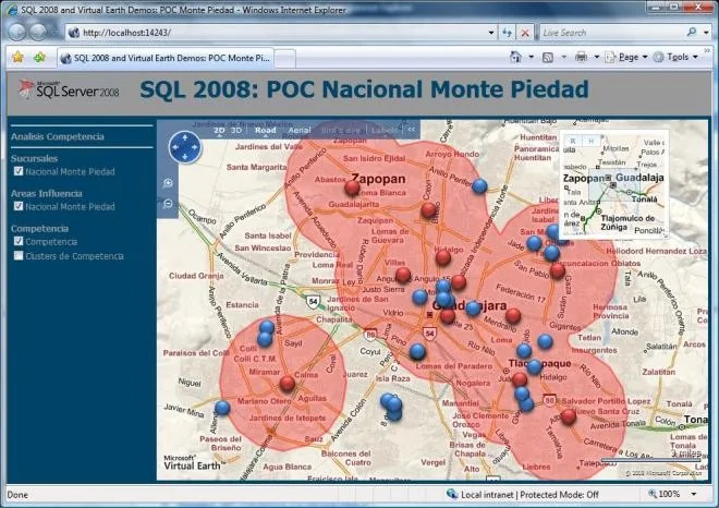One of the views from the national study: Guadalajara. Red, Monte de Piedad; blue, the competition. The blue cluster at the bottom center is a strong candidate zone.

The model didn’t decide anything. It drew a map for the people who knew the business. My part ended with the POC; Microsoft turned it into videos and demos, and I never learned where Monte de Piedad finally opened its branches, or with which model.

What stayed with me was the gravity. It was my first encounter with a gravity model outside physics: Newton’s equation, written for planets, with square meters where the mass goes and kilometers where the distance goes. And it described a street in Guadalajara well enough to argue over where to put real money. Not perfectly. Well enough. Since then I’ve believed, and I have no way to prove it, that gravity is more universal than physics: whatever accumulates pulls, and whatever is far away pulls less. I kept the screenshot and gave sessions on the SQL behind the map. And for all that belief, in my head it was a business tool. It never crossed my mind to point it at my own work, at the tables behind the map, which had a gravity of their own.

I had gravity in my hands, and I didn’t see that data has mass too.

Someone else saw it

I read Dave McCrory’s “Data Gravity” years after he published it on his blog, in December 2010. I nodded, and I forgot it. I never used the term with a client.

This year a friend brought it back. Adrian Miranda Cordero’s article “Control de costos en la nube: cuando la elasticidad se convierte en el problema” (Cloud cost control: when elasticity becomes the problem) puts data gravity first on his list of patterns behind cloud bills that grow while the business doesn’t. This time the idea landed, because I had something to set it against: ROT data, data that is Redundant, Obsolete or Trivial. The tension between those two, data gravity and ROT data, is what lit this post. Each one, on its own, explained half of what I see in today’s data platforms. I needed them pulling against each other.

McCrory’s definition, in his words:

“Consider Data as if it were a Planet or other object with sufficient mass. As Data accumulates (builds mass) there is a greater likelihood that additional Services and Applications will be attracted to this data.”

McCrory asked us to treat data as a planet, so let’s take him at his word and use Newton:

g = G · M / r²

g is the pull you feel, M is the mass (call it gigabytes), r is the distance. I’m leaving G alone. It’s a constant, and the moment you start mapping physical constants onto IT, a useful metaphor turns into pseudoscience.

Look at what’s in the equation, and what isn’t. There’s no V (Value). A petabyte of duplicated snapshots pulls your architecture exactly as hard as a petabyte of general ledger balances or transactions. And mass adds up: two bodies close together pull like one. Hold on to that. It comes back later.

I want to make the comparison explicit, because it runs through this whole series. In 2008 we drew the map of a city. Here we’re drawing the map of your data platform. The equation doesn’t change. What each letter measures does:

	Site selection, 2008	Your data platform
What pulls	A branch	A table, a model, a dataset
Mass (M)	Square meters	Gigabytes
Who gets pulled	A customer	A user, a report, a pipeline
Distance (r)	Kilometers from home to the branch	The effort to reach the data

Now picture your data platform the way McCrory asked us to, as a solar system. The lakehouse is a gas giant, and the warehouse next to it is another one. Around them orbit the data marts, smaller planets with moons of their own. And everywhere there are asteroids: the Excel files on everyone’s laptop. Each one pulls with its mass.

Two different things pull here. Mass pulls the architecture: services, pipelines, backups, cost. It doesn’t care about value. What pulls a user is something else, and we’ll get to it.

By mass, the lakehouse should win every time. It doesn’t. The Excel file on my machine weighs almost nothing, but it’s right there: I double-click and I’m in. The lakehouse is enormous, and it’s far. I have to find the right workspace, request access, wait for someone to approve it, work out which of forty tables is the one, and then learn what the columns mean. That’s r. Not kilometers, not milliseconds. Effort.

And in Newton r is squared. I won’t defend the exponent for effort, but the shape is right: distance doesn’t just weaken the pull, it crushes it. That’s how the Excel file on my laptop pulls me harder than a lakehouse with a hundred thousand times its data. And notice what nobody checks when the closest planet wins: whether the Excel file is still true. Often it’s last month’s export.

The cloud doesn’t delete. It gives you a discount.

In April 2011, four months after “Data Gravity”, McCrory published “Defying Data Gravity”, ten strategies to live with heavy data, from caching and replication to compression. Every one of them moves the data, copies it, hides it, or brings the application closer. McCrory never says it this way, but most of them are playing with r. None of them deletes anything. That’s not a criticism: he was solving latency, not governance. A year later he even named the incentive that made it worse, artificial data gravity: inbound transfer to S3 and Azure was free. Putting data in got cheaper on purpose. Deciding what to do with it didn’t.

Adrian Miranda reads the same gravity through cost. Data, he writes, “gravitates and accumulates”, a property applications don’t have: “An application server can be restarted every night without a second thought” (my translation). A data platform can’t. His storage sprawl is a list I recognized right away: historical data online by default with no retention policy, execution logs kept forever, redundant backups. That’s ROT data, the O and the R, described without the name. One of his questions for a technology director is the bridge to this post: “How much historical data is online that hasn’t been queried in the last six months?” He brings the cost. I want to add the risk.

Every row you keep is something you have to protect, something an auditor can ask you about, and something that can leak. A customer’s name, tax ID and phone number are value and liability in the same record. Most privacy laws say the same thing in different words: keep personal data only as long as the purpose that justified collecting it is still alive. When the data is relevant, the value pays for the risk. When it’s ROT data, you carry the risk and nobody collects the value. That part never shows up on the cloud bill.

There’s one more cost that never shows up on the cloud bill, and it’s r. Every ROT table in the lakehouse is one more place someone has to look, one more “which of these is the right one?”, one more message to the colleague who might know. ROT data doesn’t only weigh. It pushes the good data farther away. Your cloud provider doesn’t bill you for that effort. You pay it in payroll, by the hour, to people who were hired to use the data, not to go looking for it.

Fifteen years after McCrory’s list, the tools still sit in the same place. Cloud storage has lifecycle rules that can delete, and in the projects I’ve worked on they almost never get turned on for curated data.

So most of the time the cloud doesn’t delete. It gives you a discount. Hot to cool, cool to archive, a smaller line on the invoice, and the data stays exactly where it was in your architecture, still pulling.

And there’s a deeper problem. Storage decides by file and by date. ROT data lives in rows and in meaning.

The name

If the cloud doesn’t delete, who does? It has to be someone who can read rows and meaning, not files and dates. But before anyone can look for it, the thing they’re looking for needs a name.

I found the term this year, studying for the CDMP. The DMBOK2 (DAMA’s Data Management Body of Knowledge, 2nd edition) uses it exactly once, in chapter 1, among the implications of the data lifecycle (§2.5.9):

“Data Management efforts should focus on the most critical data: Organizations produce a lot of data, a large portion of which is never actually used. Trying to manage every piece of data is not possible. Lifecycle management requires focusing on an organization’s most critical data and minimizing data ROT (Data that is Redundant, Obsolete, Trivial) (Aiken, 2014).”

That’s all of it. (The DMBOK credits Aiken; I’m quoting the DMBOK, not him.) Three sentences were enough to hook me. Nobody seems to know who coined the term. It has been around since at least the early 2000s, and it’s at home in records management and information governance, two worlds BI barely talks to. That’s how I spent 25 years in BI without hearing it.

Back in the DMBOK, chapter 9 (Document and Content Management) has the psychology, without the acronym. One of its reasons organizations don’t remove non-value-added information: “Perceived cost of making a decision and removing physical and electronic records.” The cost of making a decision. That’s the subtitle of this series, sitting in the DMBOK.

The odd part is that I had described ROT data before I knew its name. On Halloween 2017 I wrote a post for the Primus Data blog called “La bodega de datos zombis” (The zombie data warehouse). The zombie warehouse moves, with daily or weekly loads, but the movement is automatic: “The Zombie-DW is an automaton that cannot explain why certain processes or tasks are done, nor what the value of the stored information is.” And like any zombie it feeds on its own kind: it “burns valuable resources” in IT maintenance and support (my translation, both). That’s Adrian’s cost, nine years early. In 2017 I called it a zombie. In 2026 I found out it already had a name. Less cinematic than mine, but fair enough: zombies do rot.

The same post had a sentence I saw come true again about a year ago, at a client: “even having users, this model can be a zombie, because the warehouse’s customers use it like automatons.” On a project for a large company I was responsible for one tabular model, and while checking adoption I left the filter open to see all the others. In two of them, the most active user was the developer, running weekly regression tests that compared production metrics against the new version. After eight years in production, the only “adoption” those models had was the developer’s own proof that they were still alive. The zombie was generating its own usage. The technology had changed completely since 2017. The behavior hadn’t.

Back to Mexico: Newton wasn’t enough

Back to the map. Our first iteration in Mexico was exactly the formula above, with M in square meters of branch. It wasn’t enough, for two reasons.

The first one is agglomeration. Pawnshops cluster. Five of them on the same avenue don’t behave like five small masses; customers read the street as the place you go to pawn something, and the cluster pulls harder than the five of them added up. That blue group at the bottom of the Guadalajara map is exactly that.

Remember I asked you to hold on to “mass adds up”? This is where Newton falls short, in Mexico and in data. Data agglomerates too, but what attracts is different things that belong together. Customers, purchases and products, each on its own, attract very few users. Put them together, a purchase pointing to a customer and a product, and they answer questions none of them could answer alone. The attraction jumps. In a corporation, the customers of one company attract a few users. The customers of every company, integrated in silver, attract far more.

Now cluster customer, customer_v2 and customer_old instead. They can weigh exactly the same as the integrated set. They don’t attract the same. Five pawnshops on one avenue are five real offers to compare. Three copies of the customer table are one offer and two echoes.

Picture a food court. It works because it’s agglomeration done right: tacos, sushi, pizza and a Costa Rican casado, different offers that pull harder together than the four of them added up. Now picture one where ten counters sell the same menu. One still has last year’s prices, another has a dish crossed out with tape, and nobody tells you which kitchen is still cooking. You don’t have ten options. You have one, and the job of figuring out which line to stand in.

ROT data adds to the weight of the good data, and you pay for that weight. It adds nothing to what that data can tell you.

The second reason: size alone didn’t explain attraction. Two branches of the same size didn’t pull the same. So we added what was around each one (transit stops, schools, parks, churches) and let a decision tree tell us which of those mattered. Attraction turned out to have several attributes, and it was the data, not our intuition, that picked them.

Data models have attributes too, but nobody has run that decision tree for them, not that I know of. So the list below comes from the only source I have: years of watching people adopt one model and ignore the one next to it. It’s mine, from field work, not from a paper. Take it as a first attempt:

Attribute	What it means in a data model
Names in business language	“Net Sales”, not amt_net_lcl. The user recognizes what they’re looking at.
Easy to navigate	Few tables, clear relationships. You find what you need without a map.
Explanatory metadata	Descriptions that tell you what a measure includes and what it leaves out.
Quality	The numbers are right, and they reconcile with the books.
Hides technical complexity	Surrogate keys, staging columns and load flags stay out of sight.
Relevance (signal, not noise)	It answers a question the business is asking today.

That’s the something else I promised: what attracts a user to a model isn’t its size. It’s these six. Now ask the uncomfortable question: can an old copy, the model nobody retired, attract the same way? Go down the list. The names: yes, a copy inherits them. Easy to navigate: yes, and the old model is often the simpler one. The metadata: yes, the descriptions got copied too, or were written back when they were true. Quality, the way most people check it: yes. The data was correct once, it still is, and it still reconciles with the books it came from. The one quality dimension it fails is timeliness, and nobody checks timeliness when they’re picking a model. What died is the context. Hiding complexity: yes, age has nothing to do with it. Relevance: no.

ROT data can win on five of six. The one it can’t fake is relevance: the obsolete and the trivial don’t have it, and the redundant only has it on loan from the original. That much is just the definition. What matters is that the other five, the ones you can see, can’t tell you which is which. And relevance doesn’t show up in the schema.

Dark matter: weight without light

Astronomers ran into this problem too, at a much bigger scale. Galaxies move too fast for the mass you can see. The stars at their edges orbit as if something were holding them, and with only what shines, they should fly apart. Newton, counting only the visible mass, doesn’t add up. So there has to be mass nobody can see: dark matter. It pulls like any other mass, but it doesn’t emit, absorb or reflect light. (The more academic readers will recognize Fritz Zwicky, who called it dunkle Materie in 1933, and Vera Rubin, whose galaxy rotation curves in the 1970s made it hard to ignore.)

That’s ROT data. It counts in the gravity. It keeps backups, pipelines and a developer’s regression tests in orbit, and it shows up on the bill. Your platform behaves as if it were much heavier than the data you actually use, and that’s the clue that it’s there. But it gives off no light, and by light I mean information that supports decisions. Attraction is what makes you walk over. Light is what you find when you get there. ROT data can borrow attraction, five attributes out of six. Once you’re there, it has nothing to show you. No light is a verdict about a purpose, though: not everything dark is ROT data, and that’s a post of its own.

The lesson: ROT data has mass and no light. Mass explains the cost, and the exposure. The other risk is what happens when it attracts anyway: someone, or something, picks it, and decides in the dark.

Drawing the map of a customer table

Relevance doesn’t show up in the schema. You have to measure it.

Recently I worked on an accounts receivable model for a client. The plan was the obvious one: use the same customer dimension every other model already used. A conformed dimension, in Kimball’s language. And here’s a misreading I see all the time: people take conformed to mean the same data. It doesn’t. Conformed means the same column names, the same attribute meanings and the same domain values, so a customer looks the same in every model that touches it. The rows can be identical to the full dimension, or a subset of it (for the purists, that’s Kimball’s conformance test, and it accepts both). The default is identical. Nobody asks.

Then I profiled the table, and I couldn’t make sense of it. Electronic invoicing had been mandatory for a long time. Why was a customer table this dirty? Whole blocks of strange tax IDs and odd names.

It took me a while to see it. The data wasn’t dirty. It was old. Some context, if your country doesn’t have this: in Costa Rica, an electronic invoice goes to the tax authority, which validates it, and it has to name a customer the tax authority can identify. Before it became mandatory, the old system stored whatever name the customer gave at the register, with an ID number nobody could trust. After it, a customer was someone the tax authority could find. The meaning of “customer” changed, and nobody went back to mark the records from the old regime.

Last week I wrote that meaning comes first. In that distributor, nobody had decided what a customer was. Here somebody had, and then the meaning moved, and the old records stayed where they were. Deciding once isn’t enough. Somebody has to go back.

When I measured it, about two out of every three customers in that table were ROT records. Most of the rest were good records that had nothing to do with receivables: real customers, valid IDs, no balances, no collections. The customers that actually mattered to receivables were about 4% of the table.

Those two-thirds didn’t rot with age. They rotted in one block, the day the rules changed. They’re obsolete by regime change, not by date. No rule based on creation dates would ever find them, because they aren’t files. They’re rows in a live table.

“Delete them, then.” No. The historical invoices point at those customers. There’s the gravity: correct invoices holding on to dead customers. Delete the customer and you break the invoice. And the DMBOK warns about disposing too early just as clearly as about keeping too long: some of what looks like ROT data is the record you’ll need the day after an audit.

The risk was real too, even though it never showed up on an invoice. The default sent the personal data of the whole table, names and tax IDs included, into every model, for a purpose that needed 4% of it. Nobody had approved that exposure. Nobody had been asked.

So I drew the map. If you run it on your own data on Monday, remember: it isn’t a tool for deleting. It’s for deciding.

It has two axes, and it should work on any entity with a business process behind it, not only customers.

The first axis is activity: the last business event of the process, inside a window you choose. Age is measured from the last activity, never from creation. That’s how the regime change shows up: the old records were created on a thousand different days, so creation date can’t find them. The ones that rotted went quiet once the rules changed. The ones that kept moving stay, with a label. You write the exceptions down explicitly: what’s legal or vital stays, whatever its activity. In the receivables model, accounts in legal collection got a much longer window than everything else.

One rule before you measure activity, courtesy of the zombie with one user: don’t count the activity your own systems generate. For a model, that’s the developer’s regression tests and the account that refreshes it. For a customer, it can be a lot louder. In 2008, at a retailer in Brazil, a monitoring robot logged into the website and placed an order every five minutes, invoice included, so it could raise an alert if the site or the invoicing went down. By invoice count, it was probably their most loyal customer. Activity means the business did something.

The second axis is verification, in three states: verified by an external authority (for us, the tax authority), valid format but unverified, and invalid. For most entities, the verification column needs a different authority; sometimes it’s your own master data.

(For the data quality people: invalid fails validity, verified passes accuracy, and timeliness is the activity axis’s job.)

	Verified	Valid format, unverified	Invalid
With activity	Keep. Labeled verified	Keep. Labeled unverified	Keep. Labeled invalid
No activity	Pseudonymized historical record	Pseudonymized historical record	Pseudonymized historical record

Look at what each axis decides. Activity decides whether the record stays identified. Verification decides nothing: it becomes metadata the user can see. It’s tempting to filter out the invalid IDs, or put them in quarantine. Don’t. An active customer with an invalid ID isn’t noise. It’s a signal: someone has to fix that record, and collections wants to know before they call. That’s the “explanatory metadata” attribute from the table above, doing its job.

With the map on the table, there were two cuts. The first one in the full customer dimension, the one every model uses: customers with no activity became pseudonymized historical records. The invoices still point at someone; nobody’s name or tax ID rides along anymore. (Pseudonymized, not anonymized: the tax ID is hashed with a salt we keep, so it could be reversed. We don’t.) That cut didn’t need my argument. The data protection law already asked for it, and the records from before electronic invoicing were nobody’s idea of an asset. The second one only for receivables: a dimension that conforms to the full one, same names, same meanings, same values, carrying only the customers with credit and something to collect. A cash customer is real and alive. For receivables, it’s trivial. Nothing deleted. How we built it deserves its own post later in this series; the principle fits in one line: the mass stays, the exposure goes.

The product owner signed the second one. For the wrong reasons. I was arguing governance; the business heard performance. Going from the whole table to about one customer in twenty-five changes how a model behaves, especially when the customer dimension carries dozens, even hundreds, of attributes. The model got faster, and that’s what sold it.

I’ll take it. A right decision for the wrong reason is still a decision. But think about what it means: if the model had been fast enough, nobody would have signed anything, and receivables would still be carrying the whole table to collect from 4% of it.

The lesson: whether something is ROT data gets decided by relevance, not by quality. And someone has to decide it.

Nobody drew the map

In 2008 I never found out who decided where the 80 branches went. But there was a map, and the people who knew the business had it in front of them.

Nobody ever drew the map of that customer table. Two out of every three customers rode into every model for years, and not because someone decided they should. Nobody had put the dots on a map. When someone finally did, the decisions got made: one because the law required it, the other for a reason I wouldn’t have picked.

So, how much of your data gravity is ROT data? And who decided that?

Next time we’ll come back to r, and to who chooses when the one choosing isn’t a person.

This is the first of ten posts in Who Decided That? The cloud and AI made it cheap to create, copy and keep data. They didn’t make it any cheaper to decide.